Chapter 9 Data Frames
This chapter introduces data frame objects, which are the primary data storage type used in R. In many ways, data frames are similar to a two-dimensional row/column layout that you should be familiar with from spreadsheet programs like Microsoft Excel. Rather than interact with this data structure through a UI, we’ll learn how to programmatically and reproducibly perform operations on this data type. This chapter covers various ways of creating, describing, and accessing data frames, as well as how they are related to other data types in R.
9.1 What is a Data Frame?
At a practical level, Data Frames act like tables, where data is organized into rows and columns. For example, consider the following table of names, weights, and heights:

A table of data (people’s weights and heights).
In this table, each row represents a record or observation: an instance of a single thing being measured (e.g., a person). Each column represents a feature: a particular property or aspect of the thing being measured (e.g., the person’s height or weight). This structure is used to organize lots of different related data points for easier analysis.
In R, you can use data frames to represent these kinds of tables. Data frames are really just lists (see Lists) in which each element is a vector of the same length. Each vector represents a column, not a row. The elements at corresponding indices in the vectors are considered part of the same record (row).
- This makes sense because each row may have a different type of data—e.g., a person’s
name(string) andheight(number)—and vector elements must all be of the same type.
For example, you can think of the above table as a list of three vectors: name, height and weight. The name, height, and weight of the first person measured are represented by the first elements of the name, height and weight vectors respectively.
You can work with data frames as if they were lists, but data frames include additional properties as well that make them particularly well suited for handling tables of data.
9.1.1 Creating Data Frames
Typically you will load data sets from some external source (see below), rather than writing out the data by hand. However, it is important to understand that you can construct a data frame by combining multiple vectors. To accomplish this, you can use the data.frame() function, which accepts vectors as arguments, and creates a table with a column for each vector. For example:
# vector of names
name <- c("Ada", "Bob", "Chris", "Diya", "Emma")

# Vector of heights
height <- 58:62

# Vector of weights
weight <- c(115, 117, 120, 123, 126)

# Combine the vectors into a data.frame
# Note the names of the variables become the names of the columns!
my_data <- data.frame(name, height, weight, stringsAsFactors = FALSE)- (The last argument to the
data.frame()function is included because one of the vectors contains strings; it tells R to treat that vector as a vector not as a factor. This is usually what you’ll want to do. See below for details about factors).
Because data frame elements are lists, you can access the values from my_data using the same dollar notation and double-bracket notation as lists:
9.1.2 Describing Structure of Data Frames
While you can interact with data frames as lists, they also offer a number of additional capabilities and functions. For example, here are a few ways you can inspect the structure of a data frame:
| Function | Description |
|---|---|
nrow(my_data_frame) |
Number of rows in the data frame |
ncol(my_data_frame) |
Number of columns in the data frame |
dim(my_data_frame) |
Dimensions (rows, columns) in the data frame |
colnames(my_data_frame) |
Names of the columns of the data frame |
rownames(my_data_frame) |
Names of the row of the data frame |
head(my_data_frame) |
Extracts the first few rows of the data frame (as a new data frame) |
tail(my_data_frame) |
Extracts the last few rows of the data frame (as a new data frame) |
View(my_data_frame) |
Opens the data frame in as spreadsheet-like viewer (only in RStudio) |
Note that many of these description functions can also be used to modify the structure of a data frame. For example, you can use the colnames functions to assign a new set of column names to a data frame:
9.1.3 Accessing Data in Data Frames
As stated above, since data frames are lists, it’s possible to use dollar notation (my_data_frame$column_name) or double-bracket notation (my_data_frame[['column_name']]) to access entire columns. However, R also uses a variation of single-bracket notation which allows you to access individual data elements (cells) in the table. In this syntax, you put two values separated by a comma (,) inside the brackets—the first for which row and the second for which column you wish you extract:
| Syntax | Description | Example |
|---|---|---|
my_df[row_num, col_num] |
Element by row and column indices | my_frame[2,3] (element in the second row, third column) |
my_df[row_name, col_name] |
Element by row and column names | my_frame['Ada','height'] (element in row named Ada and column named height; the height of Ada) |
my_df[row, col] |
Element by row and col; can mix indices and names | my_frame[2,'height'] (second element in the height column) |
my_df[row, ] |
All elements (columns) in row index or name | my_frame[2,] (all columns in the second row) |
my_df[, col] |
All elements (rows) in a col index or name | my_frame[,'height'] (all rows in the height column; equivalent to list notations) |
Take special note of the 4th option’s syntax (for retrieving rows): you still include the comma (,), but because you leave which column blank, you get all of the columns!
# Extract the second row
my_data[2, ] # comma

# Extract the second column AS A VECTOR
my_data[, 2] # comma

# Extract the second column AS A DATA FRAME (filtering)
my_data[2] # no comma
(Extracting from more than one column will produce a sub-data frame; extracting from just one column will produce a vector).
And of course, because everything is a vector, you’re actually specifying vectors of indices to extract. This allows you to get multiple rows or columns:
9.2 Working with CSV Data
So far you’ve been constructing your own data frames by “hard-coding” the data values. But it’s much more common to load that data from somewhere else, such as a separate file on your computer or by downloading it off the internet. While R is able to ingest data from a variety of sources, this chapter will focus on reading tabular data in comma separated value (CSV) format, usually stored in a .csv file. In this format, each line of the file represents a record (row) of data, while each feature (column) of that record is separated by a comma:
Ada, 58, 115
Bob, 59, 117
Chris, 60, 120
Diya, 61, 123
Emma, 62, 126
Most spreadsheet programs like Microsoft Excel, Numbers, or Google Sheets are simply interfaces for formatting and interacting with data that is saved in this format. These programs easily import and export .csv files; however .csv files are unable to save the formatting done in those programs—the files only store the data!
You can load the data from a .csv file into R by using the read.csv() function:
# Read data from the file `my_file.csv` into a data frame `my_data`
my_data <- read.csv('my_file.csv', stringsAsFactors=FALSE)
Again, use the stringsAsFactors argument to make sure string data is stored as a vector rather than as a factor (see below). This function will return a data frame, just like those described above!
Important Note: If for whatever reason an element is missing from a data frame (which is very common with real world data!), R will fill that cell with the logical value NA (distinct from the string "NA"), meaning “Not Available”. There are multiple ways to handle this in an analysis; see this link among others for details.
9.2.1 Working Directory
The biggest complication when loading .csv files is that the read.csv() function takes as an argument a path to the file. Because you want this script to work on any computer (to support collaboration, as well as things like assignment grading), you need to be sure to use a relative path to the file. The question is: relative to what?
Like the command-line, the R interpreter (running inside R Studio) has a current working directory from which all file paths are relative. The trick is that the working directory is not the directory of the current script file!
- This makes sense if you think about it: you can run R commands through the console without having a script, and you can have open multiple script files from separate folders that are all interacting with the same execution environment.
Just as you can view the current working directory when on the command line (using pwd), you can use an R function to view the current working directory when in R:
You often will want to change the working directory to be your “project” directory (wherever your scripts and data files happen to be). It is possible to change the current working directory using the setwd() function. However, this function would also take an absolute path, so doesn’t fix the problem. You would not want to include this absolute path in your script (though you could use it from the console).
One solution is to use the tilde (~) shortcut to specify your directory:
This enables you to work across machines, as long as the project is stored in the same location on each machine.
Another solution is to use R Studio itself to change the working directory. This is reasonable because the working directory is a property of the current running environment, which is what R Studio makes accessible! The easiest way to do this is to use the Session > Set Working Directory menu options: you can either set the working directory To Source File Location (the folder containing whichever .R script you are currently editing; this is usually what you want), or you can browse for a particular directory with Choose Directory.
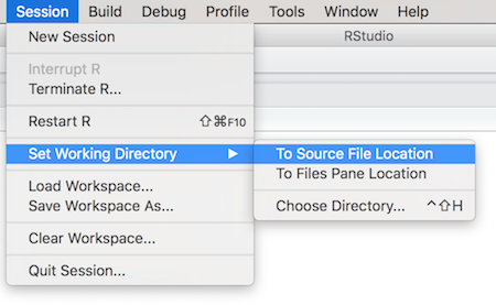
Use Session > Set Working Directory to change the working directory through R Studio
You should do this whenever you hit a “path” problem when loading external files. If you want to do this repeatedly by calling setwd() from your script to an absolute path, you may want to keep it commented out (# setwd(...)) so it doesn’t cause problems for others who try to run your script.
9.3 Factor Variables
Factors are a way of optimizing variables that consist of a finite set of categories (i.e., they are categorical (nominal) variables).
For example, imagine that you had a vector of shirt sizes which could only take on the values small, medium, or large. If you were working with a large dataset (thousands of shirts!), it would end up taking up a lot of memory to store the character strings (5+ letters per word at 1 or more bytes per letter) for each one of those variables.
A factor on the other hand would instead store a number (called a level) for each of these character strings: for example, 1 for small, 2 for medium, or 3 for large (though the order or specific numbers will vary). R will remember the relationship between the integers and their labels (the strings). Since each number only takes 4 bytes (rather than 1 per letter), factors allow R to keep much more information in memory.
# Start with a character vector of shirt sizes
shirt_sizes <- c("small", "medium", "small", "large", "medium", "large")

# Convert to a vector of factor data
shirt_sizes_factor <- as.factor(shirt_sizes)

# View the factor and its levels
print(shirt_sizes_factor)

# The length of the factor is still the length of the vector, not the number of levels
length(shirt_sizes_factor) # 6
When you print out the shirt_sizes_factor variable, R still (intelligently) prints out the labels that you are presumably interested in. It also indicates the levels, which are the only possible values that elements can take on.
It is worth re-stating: factors are not vectors. This means that most all the operations and functions you want to use on vectors will not work:
# Create a factor of numbers (factors need not be strings)
num_factors <- as.factor(c(10,10,20,20,30,30,40,40))

# Print the factor to see its levels
print(num_factors)

# Multiply the numbers by 2
num_factors * 2  # Error: * not meaningful
                 # returns vector of NA instead

# Changing entry to a level is fine
num_factors[1] <- 40

# Change entry to a value that ISN'T a level fails
num_factors[1] <- 50  # Error: invalid factor level
                      # num_factors[1] is now NA
If you create a data frame with a string vector as a column (as what happens with read.csv()), it will automatically be treated as a factor unless you explicitly tell it not to:
# Vector of shirt sizes
shirt_size <- c("small", "medium", "small", "large", "medium", "large")

# Vector of costs (in dollars)
cost <- c(15.5, 17, 17, 14, 12, 23)

# Data frame of inventory (with factors, since didn't say otherwise)
shirts_factor <- data.frame(shirt_size, cost)

# The shirt_size column is a factor
is.factor(shirts_factor$shirt_size) # TRUE

# Can treat this as a vector; but better to fix how the data is loaded
as.vector(shirts_factor$shirt_size) # a vector

# Data frame of orders (without factoring)
shirts <- data.frame(shirt_size, cost, stringsAsFactors = FALSE)

# The shirt_size column is NOT a factor
is.factor(shirts$shirt_size) # FALSE
This is not to say that factors can’t be useful (beyond just saving memory)! They offer easy ways to group and process data using specialized functions:
shirt_size <- c("small", "medium", "small", "large", "medium", "large")
cost <- c(15.5, 17, 17, 14, 12, 23)

# Data frame of inventory (with factors)
shirts_factor <- data.frame(shirt_size, cost)

# Produce a list of data frames, one for each factor level
# first argument is the data frame to split, second is the factor to split by
shirt_size_frames <- split(shirts_factor, shirts_factor$shirt_size)


# Apply a function (mean) to each factor level
#   first argument is the vector to apply the function to,
#   second argument is the factor to split by
#   third argument is the name of the function
tapply(shirts_factor$cost, shirts_factor$shirt_size, mean)
However, in general this course is more interested in working with data as vectors, thus you should always use stringsAsFactors=FALSE when creating data frames or loading .csv files that include strings.